VIEW POSTER

Material and methods

Plant material

The population evaluated in this study consists of 1,998 recombinant inbred lines (RILs) that were both genotyped and phenotyped. These were selfed for five generations (F5) in fifteen biparental crosses derived from 13 parents representing elite germplasm from throughout Southeastern breeding programs. Within this overall population, crosses with three lines, Hilliard, GA06493-13LE6, and NC08-23383, form nested association mapping subpopulations (seven, five, and four crosses, respectively). The complex subpopulations within the overall population allow high marker-density mapping of QTL for many segregating traits in the population.

The parents were selected from amongst elite Southeastern breeding lines to represent the diversity of breeding programs. While crosses were allowed to segregate for agronomically important genes such as photoperiod (Ppd) and vernalization (Vrn) genes, all parents except SS-MPV57 possess the major dwarfing allele Rht-D1b. Additionally, several parents have a Robertsonian translocation of rye (Secale cereale L.) chromosome 1: in NAM founder NC08-23383 the short arm of 1A has been replaced by the short arm of rye 1 (1RS:1AL) and the diversity parents AGS2000 and G001138-8E36 have the short arm of 1B replaced (1RS:1BL).

KASP genotyping

The thirteen parents were genotyped using Kompetitive Allele-Specific PCR (KASP) markers using standard practices^1,2 for translocations and alleles known to influence powdery mildew resistance in Southeastern germplasm. Markers that segregated between crossed parents are presented on the poster in table 1.

Genotyping

All RIL lines and founders were sequenced using genotyping-by-sequencing (GBS) with PstI and MspI restriction enzymes³. We created a pipeline in Nextflow⁴ to process data in several steps (Figure 1). The pipeline used Tassel version 5.2.95⁵ to cut barcodes, demultiplex and count sequences, and align to CS refseq v. 2.1, resulting in 751,190 variant sites. Using BCFtools v. 1.15⁶ we filtered the whole population for read depth greater than 3 and less than 100, for read quality (GQ) greater than or equal to 20, and for biallelic SNP aligned to a known chromosome, resulting in 145,911 variant sites. We used R/gaston v. 1.6⁷ to filter both marker and sample heterozygosity of less than 20% and for parent line call rates of greater than 80%. We evaluated the biparental populations separately, removing any variant sites that had less than 50% data in any biparental and keeping all variant sites that had a minor allele frequency (MAF) greater than 30% in any population, resulting in 60,466 total SNP across all lines.

Imputation of GWAS data set

To impute missing marker data we performed LD thinning in PLINK⁸, designating parents as founders and specifying parentage for all biparentals in order to create approximate population-based monotonic recombination maps for each chromosome. We split the full-population vcf into its component biparentals, then imputed missing data using beagle v. 5.4 with default parameters except the inclusion of the monotonic map⁹. We then combined the files and used gaston to merge duplicate parent lines by taking the most common call at every variant site and ensured that all markers had complete coverage. We applied LD thinning with a max r² of 0.95 and a window size of 50 Mb, resulting in 31,279 biallelic SNP markers for 1,973 lines for trait association mapping.

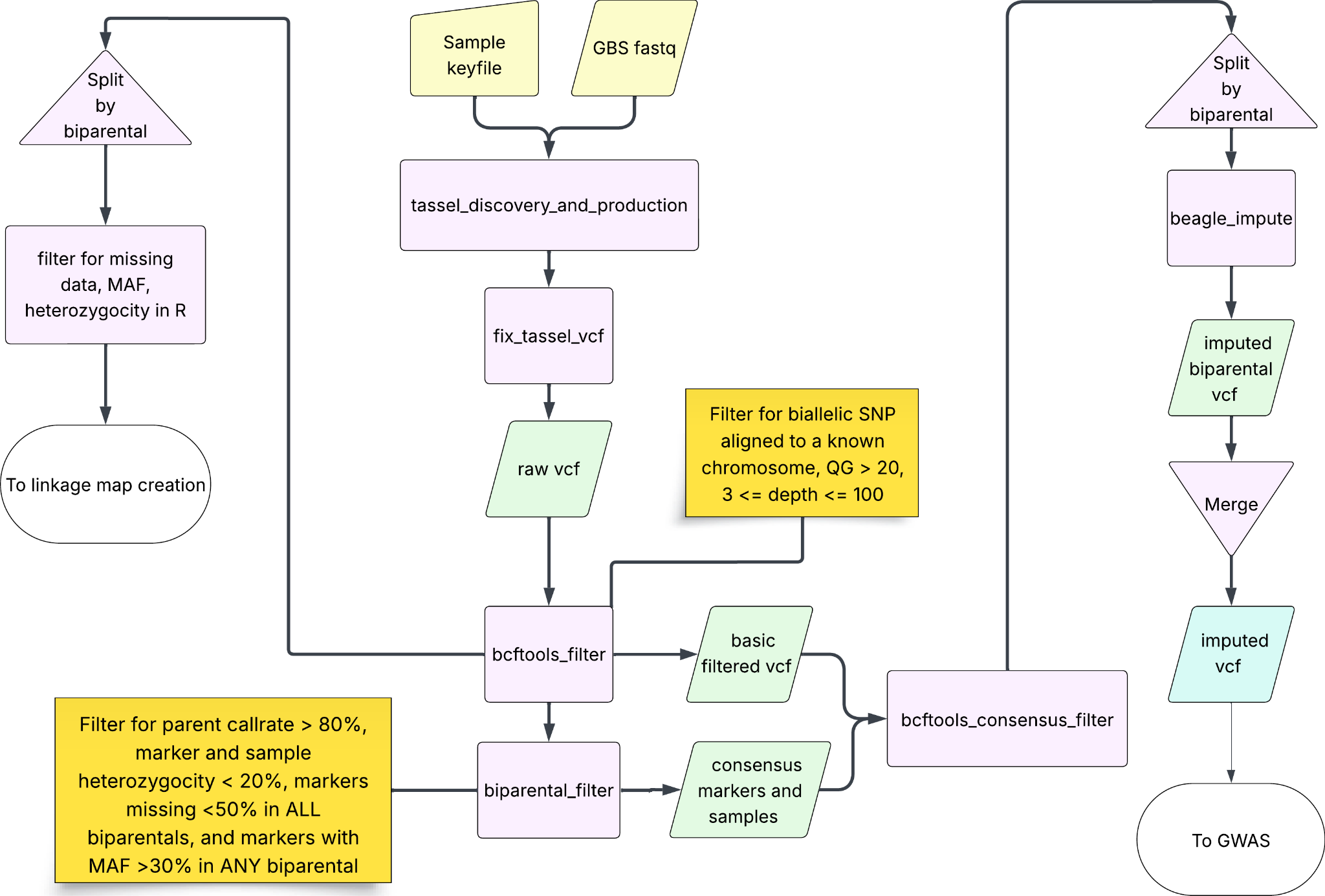
Figure 1: Diagram of genotype processing pipeline. Purple boxes represent individual processes that transform the data, yellow nodes represent input data while green nodes represent output data, the blue node represents the final product of the pipeline.

Linkage map creation

We created linkage maps for every biparental population separately. We used r/qtl and r/ASMap^10,11 to perform marker cleaning and linkage map creation. We split the SNP dataset after the first round of marker filtering (Figure 1) into biparental populations, then removed individuals with excessive amounts of missing data (between 25-50% missing, averaging 38%) and removed markers with excessive missing data (20-60% averaging 38%). Then we reduced co-located markers having identical information down to a single marker and tested those markers' segregation distortion; markers were removed if the p-value was less than the family wise error rate based on a 0.05 α Bonferroni threshold calculated using the total number of remaining markers.

Once we had clean datasets for each biparental we created linkage groups using the Kosambi function for calculating genetic distances, accepting the other default parameters in ASMap's mapmaking. For linkage group selection, we specified clustering threshold p-value between 10^-6 and 10^-13 (mean 10^-10) and selected well-formed linkage groups from the resulting bulk linkage groups. We then attempted to join linkage groups aligning to the same chromosome if multiple well-formed groups existed–if the resulting new group was less than 500 cM in length, we kept the new linkage group, otherwise the groups were kept separate. Finally, we removed singleton markers that were notably out of alignment when plotting the physical/genetic position sigmoidal curve, removing on average 20 markers per biparental.

Phenotypic evaluation:

We planted between 1,963 and 1,980 RILs from the fifteen biparental crosses at three location-year combinations: Raleigh, NC in 2022 and 2023 and in Kinston, NC in 2022. Each plot consisted of a single row one meter long, arranged in groups of four each 30 cm apart. Each group was approximately 50 cm from the next group.

We arbitrarily selected between 110 and 155 lines from each of the SunRILs biparental cross populations to be planted, depending on seed availability. Each subpopulation was assigned two blocks of 80 headrows each; each block also contained the thirteen parents and a row of barley as a marker. Individuals were randomly assigned a position within one of the two blocks. For populations with less than 132 RIL with adequate seed, RIL from larger populations were used to complete their second block. Once the blocks were constructed, we randomly assigned each block to a position in the field. This randomization procedure was followed for every planting location.

All location-year combinations had naturally occurring PM infections, with severe infections on spreader rows of hard wheat cultivar Trego surrounding the experiment and susceptible parent lines planted in every block. When infection was well established and widespread we took visual assessments of powdery mildew incidence on a 0 (no visible infection) to 4 (widespread infection extending to flagleaf) scale at a single time point near the beginning of April for each location. We measured 5,652 total observations of powdery mildew distributed between the location/year combinations, with Kinston 2022 having 1,493 observations, Raleigh, 2022 having 1,789 observations, and Raleigh 2023 having 2,370 observations. In both 2022 locations PM presence was much lower, therefore some blocks had insufficient infection for rating and were skipped. 1,998 lines total were phenotyped, with 296 being phenotyped once, 668 being phenotyped twice, and the other 1,034 phenotyped in all environments.

Statistical analysis

We gathered the raw phenotypic data from all field trials to calculate Best Linear Unbiased Estimates (BLUEs) for each individual in order to leverage our replicates, control for missing data, and account for field and location effects. Raw data was right-skewed and categorical, rather than normal and continuous, so we used a multinomial family in the model. We calculated BLUEs using ASReml, treating the genotype as a fixed effect and the Location and Year (environment) of planting as nested random effects, with a nested block effect to account for location in the field within the environment. We also calculated powdery mildew incidence as a discrete ordered categorized response variable through a cumulative logit link function¹²:

y = XbGenotype + ZuLocation:Year:Block + ε

where y is a vector of phenotypic observations for each individual genotype, b is the vector of fixed effects (genotype ID), u is the vector of random effects (environment and block), and ε is a vector of random residuals distributed as N(0, R) with R as a block-diagonal covariance matrix. X and Z are design matrices for b and u, respectively.

QTL identification

We calculated pairwise kinship scores of the whole population using R/popkin v. 1.3.23¹³ (See poster Figure 1). Population-level scores were taken by averaging the pairwise scores for each biparental cross combination.

In order to manage the strengths and weaknesses of various QTL identification methods and algorithms each trait underwent GWAS using ASRgwas¹⁴, rrBLUP¹⁵, and GAPIT's MLM, FarmCPU, and BLINK algorithms^16–18. We selected only markers that exceeded a Bonferroni significance threshold of ɑ=0.05 from each test. We performed composite interval mapping (CIM) using r/qtl2¹⁹ on each of our biparental linkage maps to identify significant markers within each biparental group. We combined all of the results of our marker trait association analysis and grouped significant markers that fell within 30 Mb of another significant marker together iteratively to collapse individual markers into loci, assigning each locus a marker range based on the position of first and last marker in locus and a peak position based on the marker with the highest LOD across models.

For all QTL identification and discussion, short arm, centromere, and long arm positions were those specified by Z. Wang et al. 2025 (20).

Works cited:

1. Rivera-Burgos, L. et al. Fine mapping of stem rust resistance derived from soft red winter wheat cultivar AGS2000 to an NLR gene cluster on chromosome 6D | Theoretical and Applied Genetics. Theor. Appl. Genet. 137, 206 (2024).

2. Semagn, K., Babu, R., Hearne, S. & Olsen, M. Single nucleotide polymorphism genotyping using Kompetitive Allele Specific PCR (KASP): overview of the technology and its application in crop improvement. Mol. Breed. 33, 1–14 (2014).

3. Poland, J. et al. Genomic Selection in Wheat Breeding using Genotyping-by-Sequencing. Plant Genome 5, (2012).

4. Di Tommaso, P. et al. Nextflow enables reproducible computational workflows | Nature Biotechnology. Nat. Biotechnol. 35, 316–319 (2017).

5. Glaubitz, J. C. et al. TASSEL-GBS: a high capacity genotyping by sequencing analysis pipeline. PloS One 9, e90346 (2014).

6. Danecek, P. et al. Twelve years of SAMtools and BCFtools. GigaScience 10, giab008 (2021).

7. Dandine-Roulland, C. & Perdry, H. Genome-Wide Data Manipulation, Association Analysis and Heritability Estimates in R with Gaston 1.5. in (KARGER, Cagliari, Italy, 2018). doi:10.1159/000488519.

8. Purcell, S. & Chang, C. PLINK 2.0.

9. Browning, B. L., Zhou, Y. & Browning, S. R. A One-Penny Imputed Genome from Next-Generation Reference Panels. Am. J. Hum. Genet. 103, 338–348 (2018).

10. Broman, K. W., Wu, H., Sen, S. & Churchill, G. A. R/qtl: QTL mapping in experimental crosses. Bioinforma. Oxf. Engl. 19, 889–890 (2003).

11. Taylor, J. & Butler, D. R Package ASMap: Efficient Genetic Linkage Map Construction and Diagnosis. J. Stat. Softw. 79, 1–29 (2017).

12. Butler, D. G., Cullis, B. R., Gilmour, A. R., Gogel, B. J. & Thompson, R. ASReml-R Reference Manual Version 4. VSN Int. Ltd (2023).

13. Ochoa, A. & Storey, J. D. Estimating FST and kinship for arbitrary population structures. PLOS Genet. 17, e1009241 (2021).

14. Gezan, S. A., de Oliveira, A. A., Galli, G. & Murray, D. ASRgenomics: An R package with Complementary Genomic Functions. VSN International (2022).

15. Endelman, J. B. Ridge Regression and Other Kernels for Genomic Selection with R Package rrBLUP. Plant Genome 4, (2011).

16. Huang, M., Liu, X., Zhou, Y., Summers, R. M. & Zhang, Z. BLINK: a package for the next level of genome-wide association studies with both individuals and markers in the millions. GigaScience 8, giy154 (2019).

17. Liu, X., Huang, M., Fan, B., Buckler, E. S. & Zhang, Z. Iterative Usage of Fixed and Random Effect Models for Powerful and Efficient Genome-Wide Association Studies. PLOS Genet. 12, e1005767 (2016).

18. Wang, J. & Zhang, Z. GAPIT Version 3: Boosting Power and Accuracy for Genomic Association and Prediction. Genomics Proteomics Bioinformatics 19, 629–640 (2021).

19. Broman, K. W. et al. R/qtl2: Software for Mapping Quantitative Trait Loci with High-Dimensional Data and Multiparent Populations. Genetics 211, 495–502 (2019).

20. Wang, Z. et al. Near-complete assembly and comprehensive annotation of the wheat Chinese Spring genome. Mol. Plant 18, 892–907 (2025).